
|
SUPPORT VECTOR MACHINESTo make these predictions, we learned about the theory and implementation of machine learning, and we focused on Support Vector Machines. This type of learning algorithm was first developed in the 1960s and became the subject of much research in the 1990s. Vapnik and colleagues, including Chervonenkis, Schölkopf, and Smola were behind these foundational developments. The algorithm, which has quickly become ubiquitous in diverse practical applications, is named for support vectors, or the data points that are used to build the model. [2]
|

THE IDEA |
Support vector machines, or SVMs, can be used for either classification or regression. Classification groups each instance into a certain class based on its attributes, and it uses as support vectors only the data points that are close to the classification boundary. Regression, on the other hand, uses the attributes to fit a function to the data, and it uses as support vectors only the points that are greater than a specified distance from this function. [2],[3] In this project, we use support vector regression to build our solar resource and power demand predictors.
The support vector regression algorithm is an optimization problem in which we want to choose a hyperplane through the data which is close to as many points as possible, such that these points are within a certain specified distance of ε from the hyperplane. It also is desired that this hyperplane is relatively flat. This leads to the minimization of a function with two terms: one describing the sum of the distances by which each point is outside of the specified ε-insensitive band, and a second term which characterizes the flatness of the function by the squared norm of w, the hyperplane’s normal. This quadratic optimization is subject to the accuracy constraints that each point is within the ε band plus or minus slack variables ξ or ξ*, to allow for points to be outside of the range. These ξ and ξ* slack variables make up the first term in the objective function. This term is multiplied by a cost parameter, C, which can be tuned to, in effect, specify the balance of the model’s accuracy versus simplicity. A large value puts an emphasis on including points within the ε band, while a small value emphasizes more having a flatter, simpler hyperplane to characterize the data. Below is Vapnik’s 1995 formulation of the problem, which can be solved by formulating its dual. For this, a kernel trick is used, which maps the data to a higher dimension to find a solution. A common kernel, and the one which we used, is the radial basis function. It has an adjustable parameter, γ. [2]-[4] |
|
We can change the fit of the model to the data set by varying the parameters ε, C, and γ. According to Müller et al., these parameters, though “powerful means for regularization and adaptation to the noise in the data,” are difficult to select. The lack of a simple, general method or theoretical bounds for their selection shows that this is an area of support vector machines with potential for growth. [3] In our project, we used a simple grid search algorithm which built models by varying C and γ through a specified range and compared the error of each model in a cross-validation. Parameter selection aims to achieve the balance between over- and under-fitting. Under-fitting the data results in a model that does not capture all the characteristics of the set, while over-fitting builds a model that captures the individual peculiarities or noise of the given data so well that it is not useful for predicting future behavior. In our tests for power load profile parameters, the best results came from C=1024 and γ=7. For the solar resource, we found C=256 and γ=4 to perform well.
|
PARAMETER SELECTION |
IMPLEMENTATION |
Support Vector Regression can be implemented in several ways. A common package which is available for use in MATLAB and Java is called LibSVM. We implemented it in both MATLAB directly and in Java through a programming interface called Weka, which organizes the training and testing process and gives the capability to filter the data, such as normalizing the attributes, which is important to ensure that each is given equal weight. In the preliminary stages of experimenting with regression techniques, we worked with several data sets, including detailed weather information readily available from the National Renewable Energy Laboratory for a typical meteorological year at many locations around the country and historical hourly data from a network of weather stations in the northwest U.S. available from the Bureau of Reclamation. The latter source of data proved to be the most useful, as it is continuously updated and includes many attributes that are important for predicting solar radiation. Detailed power load information from southern Washington, northern Oregon, and western Idaho was also available from the Bonneville Power Administration Balancing Authority. For making predictions, we obtained forecasted weather attributes from the National Weather Service. |
|
To build a predictor for solar radiation, we obtained hourly weather data from January 2010 through March 2015. The attributes in this data were the day of the year, time, temperature, relative humidity, wind gust speed, and wind speed. The target value was the global horizontal irradiance, or GHI, which describes the solar radiation incident on a flat photovoltaic panel. We took data from weather stations at five locations: Imbler, Powell Butte, Echo, and Baker Valley in Oregon, and George in Washington. These locations are shown by the red markers in Figure 2. The solar radiation showed notable variance across locations and hour-to-hour in each location. At a glance, it seemed that this variance was greater than that of the sunniest region of the country, southern California and Arizona, which suggests that a reliable solar predictor could be important in an area such as this one. To build the power load predictor, we used hourly weather and power load data from January 2007 to March 2015. The power load does not correlate strongly with as many features as the solar radiation. Successful peak-load predictors have been built using only date and time as attributes. [4] For this project’s aim to predict the hourly load, we found it beneficial to include temperature data from two locations: Hood River, OR, and Boise, ID, shown in teal in Figure 2. It is important to note that the power load generally follows a slightly different pattern on weekends. We included a binary attribute that describes whether or not the day is a weekend. In addition, the temperature tends to have the opposite effect on the power load depending on whether the date is between roughly the beginning of April and the end of September. [4] We added a binary attribute describing this. The other attributes were the year, day, time, temperature at Hood River, and temperature at Boise. The target value was the power load in MW. |
BUILDING THE PREDICTORS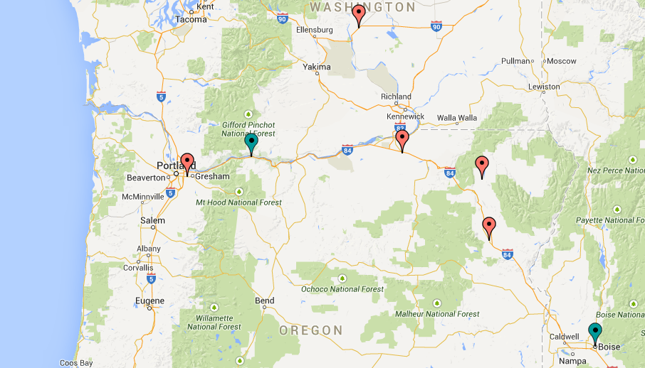
The weather stations. The red markers indicate locations for solar forecasting, and the blue markers indicate temperature data sources for power load forecasting.
|
